Workflow overview
General workflow
ARC3O simulates brightness temperatures from climate model output. It follows the following workflow.
Note
Please remain aware that the assumptions used in ARC3O have only been evaluated for the frequency of 6.9 GHz, vertical polarization at the moment! The use for other frequencies and polarizations is at your own risk!
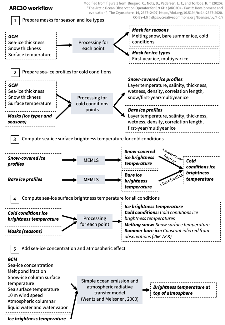
Step 1: Prepare masks for season and ice types
In [Burgard et al., 2020a] and [Burgard et al., 2020b], we show that different approaches are needed to simulate the sea-ice surface brightness temperatures
depending on the ice type (first-year or multiyea ice) and on the “season” (cold conditions, melting snow, bare ice in summer). This is why,
in a first step, ARC3O creates masks to divide the grid cells into those criteria. This is done in the main function with
arc3o.core_functions.prep_mask().
To divide the grid cells into different ice types, the function arc3o.mask_functions.ice_type_wholeArctic()
uses the time series of the sea-ice thickness to determine if there was ice in the grid cell in the year preceding each timestep,
thus dividing into open water, first-year and multiyear ice.
To divide the grid cells into the different seasons, the function arc3o.mask_functions.define_periods() uses information about
sea-ice thickness, snow thickness, and surface temperature to identify periods of melting snow and periods of bare ice in summer. All
other grid cells are defined as “cold conditions”.
The resulting masks are written to period_masks_assim.nc in outputpath.
Step 2: Prepare sea-ice profiles for cold conditions
In a second step, we prepare the climate model output data for the simulation of the ice surface brightness temperature
for cold conditions through the Microwave Emission Model for Layered Snowpacks (MEMLS, [Wiesmann & Matzler, 1999] and [Tonboe et al., 2006]).
This is done in the main function with arc3o.core_functions.prep_prof().
Based on the climate model sea-ice thickness, snow thickness, and the snow/ice surface temperature, combined with the masks
described in Step 1: Prepare masks for season and ice types, ARC3O adds the dimension layer_number to the lat-lon-time arrays. This way, it prepares two sets
of profiles (ten ice layers and one snow layer), one set for snow-covered ice and one set for bare ice (see arc3o.profile_functions.create_profiles()). These profiles
describe the layer:
temperature
arc3o.profile_functions.build_temp_profile()correlation length
arc3o.profile_functions.build_corrlen_profile()type
arc3o.profile_functions.build_sisn_profile()
The resulting profiles are written to profiles_for_memls_snowno_yyyymm.nc and profiles_for_memls_snowyes_yyyymm.nc
in outputpath.
Step 3: Compute sea-ice surface brightness temperature for cold conditions
In a third step, the two sets of profiles prepared in Step 2: Prepare sea-ice profiles for cold conditions are used to simulate the brightness temperature at the surface of
the snow and ice column, through the Microwave Emission Model for Layered Snowpacks (MEMLS, [Wiesmann & Matzler, 1999] and [Tonboe et al., 2006]).
This results in two sets of brightness temperatures (one set for snow-covered ice and one set for bare ice). They are then
combined, weighted by the bare-ice fraction given by the climate model output. This step is done in the main function with
arc3o.core_functions.memls_module_general().
The MEMLS simulation is conducted through calling the function arc3o.core_functions.run_memls_2D(). More details about
the detailed steps of the brightness temperature simulation can be found in arc3o.memls_functions_2D.memls_2D_1freq()
and its documentation of memls_functions_2D.
The resulting ice surface brightness temperatures for cold conditions are written to TB_assim_yyyymm_f.nc in outputpath,
where f is the rounded frequency of interest.
Step 4: Compute sea-ice surface brightness temperature for all conditions
In a fourth step, the ice surface brightness temperatures are extended to other seasons than “cold conditions”, i.e.
to the seasons “melting snow conditions” and “bare ice in summer conditions”. This step is done in the main function with
arc3o.core_functions.compute_TBVice() and arc3o.core_functions.compute_emisV().
Note
Please remain aware that, currently, the brightness temperatures of “melting snow conditions” and “bare ice in summer conditions” are set to the values for 6.9 GHz, vertical polarization, for all frequencies and polarizations! This is because we concentrated our effort on 6.9 GHz, vertical polarization. You are welcome to try out new things though! :)
Step 5: Add sea-ice concentration and atmospheric effect
In a fifth step, the contribution of the ocean and melt ponds to the surface brightness temperature (through the sea-ice concentration
the melt-pond fraction, the snow/ice surface temperature, the sea surface temperature and wind speed) is included. The resulting
surface brightness temperature (combining ice and open water brightness temperatures) is used as an input as a
surface brightness temperature for a simple atmospheric radiative transfer model. This radiative transfer model additionally
requires the atmospheric columnar liquid water and water vapor.
Both adding the oceanic contribution and adding the atmospheric contribution are done in the main function with arc3o.core_functions.amsr(),
based on the geophysical model described in [Wentz & Meissner, 2000].
The resulting top-of-the-atmosphere brightness temperatures for all grid cells are written to TBtot_assim_yyyymm_f.nc in outputpath,
where f is the rounded frequency of interest.